
The 2025 Ohio State Quantathon was a five-day team competition with one question: each day, how much money should sit in the S&P 500 and how much in bonds, if the goal is to beat buy-and-hold? Our answer was QuantifyAI. It labels every day Bear, Bull or Static with a 20% drawdown rule, predicts that label 63 trading days ahead with gradient boosting, flags unusual days with an anomaly ensemble, and backtests about ten allocation strategies on top of both.
Over 2019 to 2022 the best strategy returned 56.68% with a Sharpe ratio of 1.10 and a maximum drawdown of -10.68%, against 52.97%, 0.58 and -33.92% for buy-and-hold. The more interesting part is where that Sharpe comes from. Annualised return barely moves, 11.88% against 11.21%, while annualised volatility falls from 22.9% to 10.7%. The strategy wins by holding less equity through a window that contains the 2020 crash. It is a risk-control result more than a forecasting one.
Why It Matters
The competition gave us a daily S&P 500 series, a bond rate and two "market-based probability" series. The brief asked us to predict market regimes, comparing Markov chains, gradient boosting and LSTMs, and to beat buy-and-hold. This post covers the gradient boosting path.
Regimes are a useful target because allocation needs only one decision a day, how much equity to hold. A coarse label like Bear, Bull or Static maps straight onto that decision. Our first attempt, predicting the price level itself, went nowhere (see Problems).
What makes this worth writing up is the gap between the Sharpe and the forecast. A strategy that cuts equity at the right moments looks brilliant on Sharpe whether or not its model can see the future, because Sharpe rewards lower volatility as much as higher return. If you want to know what you built, you have to pull the two apart, and that is what the experiments below do.
Technical Details
Regimes From a Drawdown Rule
The label is backward-looking. For each day, take the rolling 252-day maximum and minimum of the S&P 500. Let
A day is Bear if
Predicting a Regime 63 Days Out
The classifier predicts the label 63 trading days ahead, roughly one quarter. The model is scikit-learn's gradient boosting [2], which fits trees stage by stage to the gradient of the loss. Features are about 24 engineered columns from the two probability series, S&P returns and volatility, and bond-rate features.
Financial time series need evaluation that respects time [3], so the model trains on 2007 to 2018 and is scored on 2019 to 2022. A slow-moving label also needs a persistence baseline. If the regime rarely changes, "it stays the same" is hard to beat.
Sharpe and What It Rewards
The Sharpe ratio is mean return over standard deviation, annualised by
Anomaly Detection as an Ensemble
The anomaly module runs IsolationForest [7], DBSCAN [8] and a z-score, normalises each score, and takes the mean. A percentile of that mean, set by a contamination fraction, decides which days are flagged. The fraction fixes how many days get flagged: at contamination=0.03, 31 of the 1,008 test days.
Architecture
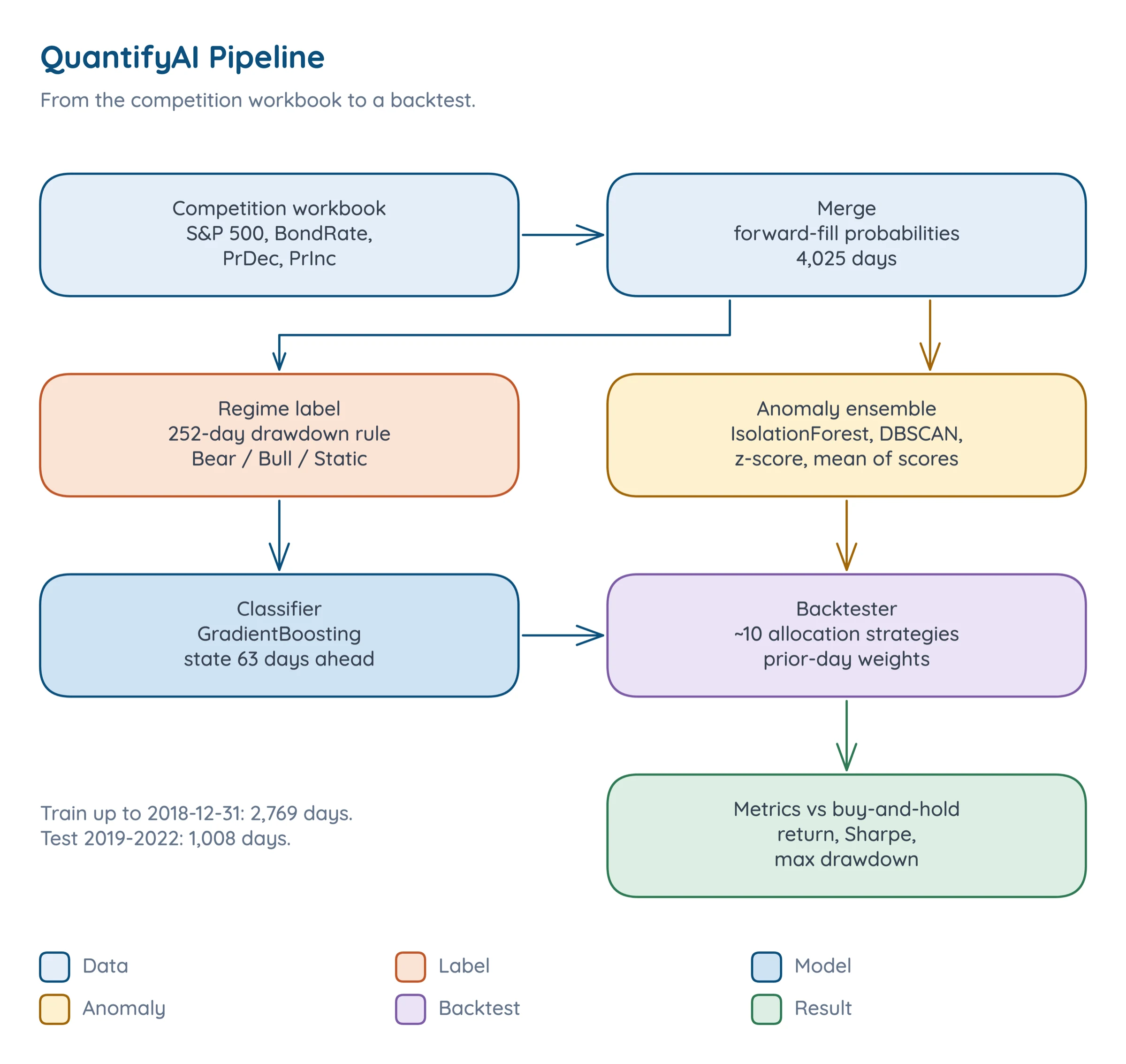
Two paths do the work. The label feeds the classifier, and the merged features also feed the anomaly ensemble. The backtester combines both, turns them into daily stock and bond weights, and compares each strategy to buy-and-hold. Every strategy applies the previous day's allocation to today's return, so the portfolio timing is causal. Rebalancing is daily, there is no leverage, and bonds earn the supplied rate.
Implementation
The code excerpts below are from the team repository, SadeekFarhan21/QuantifyAI.
The Regime Label
This is the core of classify_markets.
df['Rolling_Peak'] = df['SP500'].rolling(window=window, min_periods=1).max() |
On the merged 4,025 days the rule gives 8.2% Bear, 43.0% Bull and 48.8% Static. Over 2019 to 2022 the counts are 72 Bear, 599 Bull and 337 Static.
The Classifier
The classifier's target is the state shifted forward by 63 rows.
df['Future_Market'] = df[target_col].shift(-forward_periods) |
Grid search over n_estimators 100 or 200, learning rate 0.05 or 0.1 and depth 3 or 4 picked learning rate 0.1, depth 3 and 200 estimators, with subsample 0.8 and min_samples_split 5 fixed.
The Anomaly Ensemble
The threshold is a percentile of the ensemble score.
df['ensemble_score'] = normalized_scores.mean(axis=1) |
Over the test period it flags 31 days: Anomaly distribution: {1: 977, -1: 31}.
Causal Portfolio Timing
Every strategy uses the same loop. Yesterday's weights earn today's returns, so no strategy trades on a price it hasn't seen yet.
sp500_contrib = df['SP500_Allocation'].iloc[i-1] * df['SP500_Return'].iloc[i] |
The Headline Strategy
The combined anomaly and regime strategy holds 1.0 equity in Bull, 0.5 in Static and 0.0 in Bear. A flagged day sends it to 0% equity, and it recovers linearly over 10 days. Its other parameters:
recovery_period = params.get('anomaly_recovery_period', 10) |
Who Built What
Jalen Francis built the modular pipeline, including the backtester. My parts were the data merging, an early modelling notebook, the slides, most of the paper's text and TikZ figures, and the feature-importance plotting and accuracy logging. Aditya Bhati wrote an early abstract draft, and Jayson Clark is a co-author on the paper and slides.
Problems
1. A Price Regression That Went Nowhere
My first attempt, before the pipeline existed, was a linear regression from the bond rate and the two probability series to the S&P 500 level, trained to 2018-12-31 and tested from 2019. On the test years it had a mean squared error of 6,078,269.9 and an R-squared of -7.147, far worse than predicting the mean. Those inputs cannot predict a price level, and that dead end is why the project switched to classifying regimes. A regime is a coarser target, and it is the one an allocation rule needs anyway.
2. Two Sheets on Different Calendars
The price sheet has 4,527 daily rows. The probability sheet has 736 rows on irregular dates. They merge to 4,025 days from 2007-01-08 to 2022-12-30, which means most days need a probability value carried from somewhere. The loader forward-fills, so every day sees the most recent probability that already existed.
3. Telling Risk Control From Forecasting
A Sharpe of 1.10 against 0.58 looks like a model that sees the future. But the same number comes out of any rule that happens to hold less equity during a crash. Sharpe alone can't tell you whether a de-risking strategy has skill. The way through was to change one input at a time on the same test frame, add a random-flag placebo and simple constant mixes, and put a persistence baseline next to the classifier. That is the experiment below.
Experiments
The experiments use the default pipeline with the enhanced backtester, trained on 2,769 days up to 2018-12-31 and tested on the 1,008 days of 2019 to 2022. Each ablation changes one input at a time on that same test frame:
- Anomalies switched off.
- A causal detector, flagging days where the return is more than 3 standard deviations from its trailing 252-day mean, which flags 30 days.
- A placebo: 31 random days flagged as anomalies, 200 runs.
- Predictions replaced by always Bull, with and without the real anomalies.
- Predictions replaced by the current true state.
- Constant 50/50 and 60/40 stock and bond mixes.
- Out-of-sample accuracy of the model's
Predicted_Marketand a persistence baseline, on 2019 to 2022 only.
The test is a single path with one crash in it, and the placebo is the only uncertainty estimate I have.
Results
Against Buy-and-Hold
Buy-and-hold returned 52.97% in total, 11.21% a year, with a Sharpe of 0.58, a drawdown of -33.92% and a win rate of 54.12%. The combined anomaly-regime strategy reaches a Sharpe of 1.10, with 56.68% total, a drawdown of -10.68% and a 59.03% win rate. The prediction strategy returned 42.77% and the dynamic strategy 51.65%.
Against simple baselines on the same window, a constant 50/50 mix returned 29.79% with Sharpe 0.63 and drawdown -18.03%, and 60/40 returned 34.70%, 0.61 and -21.38%. Only the headline strategy beats buy-and-hold on total return, and buy-and-hold has the deepest drawdown of any of them. The window contains the 2020 crash, the fast recovery and the 2022 fall, which is exactly the kind of period where cutting equity pays.
A Sticky Label Is Hard to Forecast
On the 1,008 test days, with the model trained only to 2018-12-31, its Predicted_Market matches the same-day state 60.6% of the time and the state 63 days ahead 56.8%. Predicting that the state simply stays the same for 63 days scores 73.4%. Regimes are sticky, and the edge in the backtest doesn't come from seeing a quarter ahead. The model also leans Static: its predicted mix over the test period was 664 Static, 264 Bull and 80 Bear days, against true counts of 599 Bull, 337 Static and 72 Bear.
What the Ablations Say
- A simple trailing detector does at least as well as the ensemble. Flagging 3-sigma days against a trailing 252-day mean gives 58.63% total return, Sharpe 1.16, drawdown -10.58%.
- The detector's timing is not clearly skill. Flagging 31 random days gives a mean total return of 43.01% (5th to 95th percentile 28.36 to 58.69) and a mean Sharpe of 0.93 (0.65 to 1.22). 14.5% of placebo runs match or beat the Sharpe of 1.10, and 7% beat the total return.
- The predictor and anomaly flags together are what cut drawdown. Always Bull with the real anomalies has a drawdown of -22.56%, and always Bull with none has -29.01%, against -10.68% for the headline strategy. But replacing predictions with the current true state gives 50.35%, Sharpe 0.88 and drawdown -19.55%, so the evidence that the machine-learned prediction adds value beyond simple rules is weak.
De-risking paid off in a period that contained a crash, and I can't separate the model's skill from the schedule of when equity was cut. That is the claim the numbers support.
What I Would Change
Always Report the Persistence Baseline
For a label that changes rarely, "stays the same" is a strong baseline. A model that loses to it has learned less than it appears to.
Test on More Than One Path
A single 2019 to 2022 path with one crash cannot support a claim of skill. Next time I would keep a second window that is never used for choosing a strategy, score the final number there, and count how many variants were tried [5][6].
Run the Placebo First
The random-flag placebo is what showed the detector's timing is not clearly skill. I would run it before writing any claim about detector timing.
References
- Adrian Pagan and Kirill Sossounov. A Simple Framework for Analysing Bull and Bear Markets. Journal of Applied Econometrics, 2003.
- Jerome Friedman. Greedy Function Approximation: A Gradient Boosting Machine. Annals of Statistics, 2001.
- Marcos Lopez de Prado. Advances in Financial Machine Learning. Wiley, 2018.
- William Sharpe. The Sharpe Ratio. Journal of Portfolio Management, 1994.
- David Bailey and Marcos Lopez de Prado. The Deflated Sharpe Ratio: Correcting for Selection Bias, Backtest Overfitting and Non-Normality. Journal of Portfolio Management, 2014.
- David Bailey, Jonathan Borwein, Marcos Lopez de Prado and Qiji Jim Zhu. The Probability of Backtest Overfitting. Journal of Computational Finance, 2017.
- Fei Tony Liu, Kai Ming Ting and Zhi-Hua Zhou. Isolation Forest. IEEE International Conference on Data Mining, 2008.
- Martin Ester, Hans-Peter Kriegel, Jorg Sander and Xiaowei Xu. A Density-Based Algorithm for Discovering Clusters in Large Spatial Databases with Noise. KDD, 1996.