
Columbus runs LEAP, a loan fund that pays for replacing lead and galvanized water service lines. It lends up to $10,000 at 0% for up to 99 years, and the loan is repaid in one lump sum when the house is sold or equity is withdrawn. For Quantathon 2026 (the SIAM-MTI challenge), Aaditya and I had to answer one question: how much should the city set aside in 2026 so the fund never runs dry before the 2037 federal replacement deadline?
We built a cohort Monte Carlo that simulates 34,269 eligible lines over twelve years on 3,000 paths and takes the 95th percentile of each path's worst cumulative deficit. The answer is $2.73M for loans, against $4.01M for an equivalent grant program. A Markov-chain benchmark built from the same inputs agrees with the simulation to within 0.015% once both measure the same quantity. The more useful finding is where the uncertainty lives. The sampling error on $2.73M is about $25k, while a plausible range for a single uptake rate estimated from the pilot moves it by nearly $1M.
Why It Matters
Lead service lines have a hard federal deadline, and a loan fund that runs out of money halfway there stalls replacements for the households that depend on it. A grant program is simple to budget, because you spend what you give away. A loan fund is harder, because money comes back, but slowly and at times nobody controls. A loan is repaid when a house sells, and nobody knows when that will be.
The task asked for the 2026 upfront funding that sustains the program through 2037 at a 95%-sufficient level, a comparison of the loan structure with a grant, and a confidence interval on the recommendation. There are 34,269 eligible lines (whole-lead lines plus customer-side galvanized lines, minus the overlap) out of 288,389 in the system materials table. The pilot data is tiny, with 64 observed funded loan amounts with a mean of $7,386 and a cap-limited maximum of $10,000, and a snapshot of 62 active loans (42 completed, 20 in progress).
That set the design. A city cannot observe a fund's future, so the reserve has to come from a simulation of household behavior over twelve years, driven by parameters estimated from a pilot that is barely larger than a classroom. A single expected value would hide the risk, so the model produces a distribution and reports a high percentile of it. Everything else we built is there to show how far to trust that percentile.
This was a two-person team entry. Aaditya wrote the core cohort Monte Carlo and the first versions of the assumptions, charts, data loading and report driver. I built the cross-checks around it (the Markov chain, the deterministic benchmark, the bootstrap, the tornado analysis, stress tests and NPV), the ML-enhanced agent simulation, the paper and the slide deck.
Technical Details
Reserve as the Peak of a Cumulative Deficit
Let
For grants,
Loans as a Three-State Chain
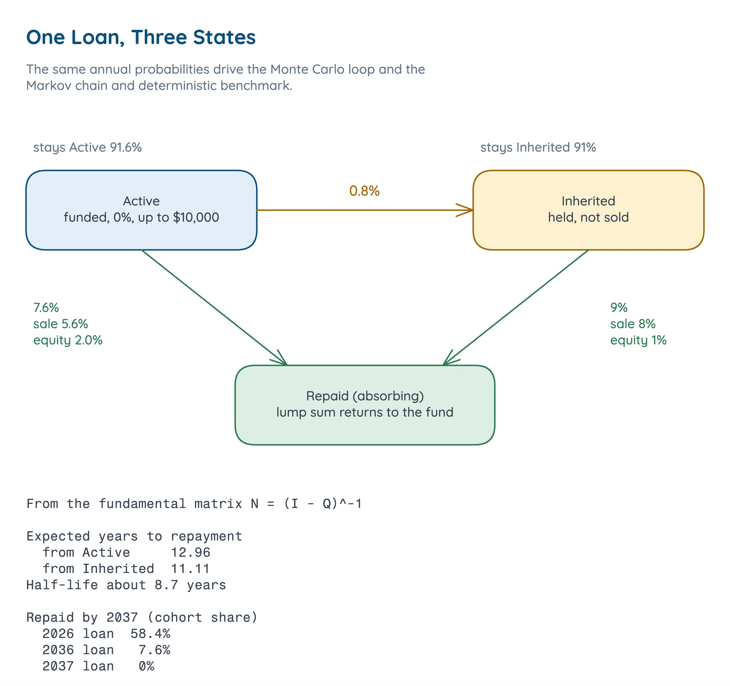
Each loan is Active, Inherited or Repaid. Active loans repay on a sale (5.6% a year) or an equity withdrawal (2.0%), and become Inherited with probability 0.8%. Inherited loans repay at 8% (sale) plus 1% (equity). That is an absorbing chain, and its fundamental matrix
Jensen's Inequality for a Maximum
For any random process,
Two Kinds of Uncertainty
The bootstrap [3] resamples the simulated paths and tells you how precisely a finite number of paths pins down a statistic. It says nothing about whether the parameters that generated the paths are right. Parameter uncertainty needs a different tool, such as one-at-a-time sweeps [4] or sampling parameters from priors.
Architecture
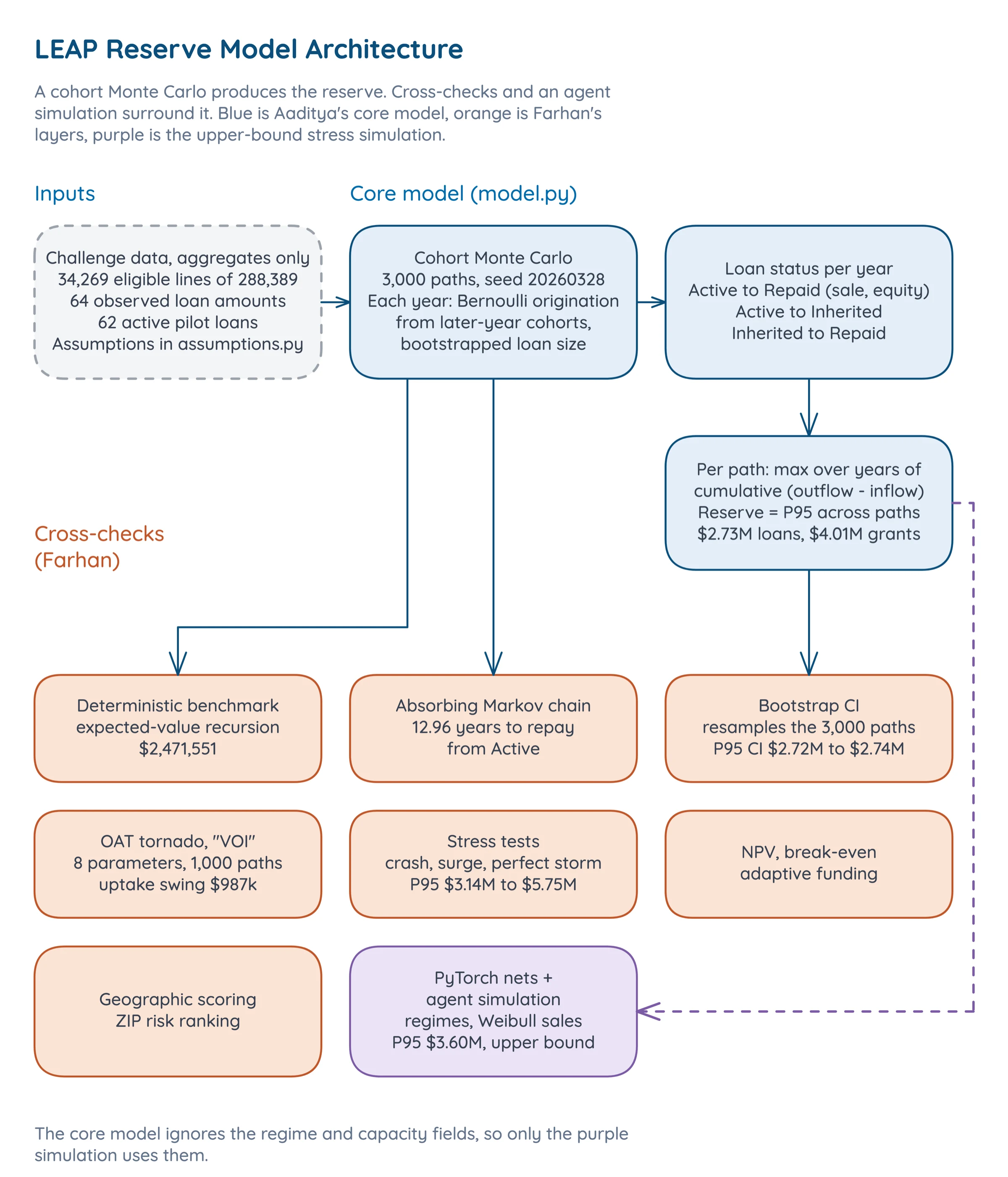
The core is Aaditya's chain of three steps: simulate originations and loan status per year, take each path's maximum cumulative deficit, and report the 95th percentile. My cross-checks sit around it. The ML-enhanced agent simulation is a separate, richer model that adds a regime-switching housing market and contractor capacity, and we treat its answer as an upper bound.
Implementation
The Cohort Monte Carlo
This part is Aaditya's, and I quote only the mechanism in condensed form. The 34,269 lines are spread across 2026 to 2037 by fixed schedule weights. Each year, every not-yet-replaced line in a later scheduled cohort originates a loan with probability
# condensed from solution/model.py (Aaditya): type hints removed, a local inlined |
Loan sizes are bootstrapped from the 64 observed amounts and inflated 3% a year. Then each active loan draws once a year against the sale, equity and inheritance probabilities above. The per-path requirement is the running maximum of cumulative outflow minus inflow, and the recommendation is its 95th percentile over paths.
The Markov Chain and Deterministic Benchmark
The transition matrix is built from the same scenario probabilities, so the deterministic model and the Monte Carlo cannot disagree because of different inputs.
# solution/markov.py |
From it I derive an expected 12.96 years to repayment from Active and 11.11 from Inherited (standard deviations 12.29 and 10.60), a half-life of about 8.7 years, and the fraction of each origination year's cohort repaid by 2037: 58.4% for a 2026 loan, 7.6% for 2036 and 0% for 2037. Money lent late in the program barely comes back before the deadline.
The Cross-Check Stack
The bootstrap resamples the 3,000 path-level requirements 2,000 times with seed 42. The tornado varies eight parameters one at a time, at the optimistic and conservative values of two hand-chosen scenarios, with 1,000 paths per variant. The stress tests and the NPV analysis each reuse the core simulator.
The ML-Enhanced Simulation
The agent simulation scales 10,000 parcels up to 34,269 and adds regime switching (Boom, Normal, Recession with 70% persistence), a Weibull sale hazard, a deadline urgency ramp, contractor capacity, and a 4% return on the fund. Two networks, UptakeNet and SaleHazardNet (12 features, a 64-32-16 MLP, 150 epochs of Adam), supply per-parcel probabilities. They are smooth interpolators of heterogeneous assumptions: they map parcel features to per-parcel probabilities, the kind of function an MLP of this shape can approximate closely [5]. On the 10,000 v4 parcels they reproduce their targets with correlations of 0.9969 (uptake) and 0.9726 (sale).
Problems
1. A Cross-Check That Looked Like a Failure
The deterministic benchmark gives a maximum cumulative deficit of $2,471,551. The Monte Carlo mean is $2,489,537, a gap of 0.72%, and the deterministic value falls outside the bootstrap interval for the mean, $2,484,206 to $2,494,821. Two implementations built from the same inputs should not disagree like that, so either one has a bug or the comparison is wrong.
It was the comparison. The deterministic model computes
# max of the averaged curve, against the mean of per-path maxima |
The result is $2,471,915, within 0.015% of the deterministic $2,471,551. Compared on the same statistic, the two independent implementations agree to four significant digits. The gap that remains is Jensen's inequality, and it comes from the peak year moving between paths: 1 path peaks in 2031, 47 in 2032, 618 in 2033, 1,616 in 2034, 699 in 2035 and 19 in 2036.
2. Separating Sampling Error from Parameter Uncertainty
The bootstrap interval for the P95 is $2,716,604 to $2,741,433, a width of about $24.8k. That is tight, and it is easy to read as the precision of the $2.73M. It is only the Monte Carlo sampling error from using 3,000 paths instead of infinitely many. The tornado swing on the uptake start rate alone is $987,296 (P95 of $2.21M at 0.16% to $3.20M at 0.25%), about 40 times the P95 interval width and 93 times the mean interval width. A confidence interval on the recommendation is mostly parameter uncertainty, with sampling error a small part of it.
The rate itself, 0.20% a year, rests on a single pilot window of 62 active loans. To make the point concrete I pooled paths over a uniform prior on the uptake start rate from 0.16% to 0.25%, the tornado's own range. The prior is my assumption. The mixture has a mean of $2,514,853 and a P95 of $3,029,090. Treat that as an illustration of how much wider an honest interval is, not as a better estimate.
Experiments
Each experiment varies one thing against the same core simulator:
- The base run (3,000 paths, seed 20260328), which produces the headline.
- The Jensen decomposition and peak-year histogram from those same paths.
- The bootstrap interval (2,000 resamples, seed 42).
- An uptake start-rate sweep at seven values, 500 paths each, holding the cap (0.30%) and growth (5%) at their base values.
- A pooled mixture over an assumed uniform prior on the start rate, 10 grid points times 300 paths, seed 7.
- The three stress scenarios, 1,000 paths each, seed 20260401.
- A 1,000-path run on the organizer-supplied v4 parcel file.
Results
The Headline
With 3,000 paths and seed 20260328 the loan requirement has a mean of $2,489,536.59, a median of $2,488,412.51, a P95 of $2,731,561.30, and a P2.5 to P97.5 spread of $2,201,801 to $2,771,970 (minimum $2.02M, maximum $3.09M). The grant mean is $3,708,633 and its P95 is $4,005,262, so the loan structure saves $1.27M at the P95. A full run takes 21.4 seconds of pure Python. Across the three scenarios, the loan P95 is about $2.01M (optimistic), $2.73M (base) and $3.49M (conservative), against $3.16M, $4.01M and $4.77M for grants.
The Averaged Curve and the Peak Year
The averaged deficit curve peaks at $2,471,915 in 2034, and paths peak anywhere from 2031 to 2036, mostly 2033 to 2035. That spread in peak years is the whole Jensen gap.
One Assumption Dominates
The P95 is roughly linear in the uptake start rate until the cap binds: $1.45M at 0.10%, $2.09M at 0.15%, $2.21M at 0.16%, $2.73M at 0.20%, $3.20M at 0.25%, and $3.35M at both 0.30% and 0.40%. That is about $1.3M of reserve per 0.10 percentage points of uptake. The 0.10% to 0.20% endpoints, $1.45M to $2.73M, give $1.28M. The tornado ranking puts uptake first, then schedule weighting, then sale probability and cost inflation. Federal rules could raise uptake by 2 to 5 times, which would move the reserve toward the surge scenario.
Stress Scenarios
On 1,000 paths the base P95 is $2,728,307. The 2029 Housing Crash, which moves the sale and equity probabilities, is $3,139,293 (+14.9%). Surge Uptake, which moves the trigger start, cap and inflation, is $4,975,191 (+82.1%), and Perfect Storm is $5,754,568 (+110.7%). The mean increases over the base mean are +15.7%, +87.4% and +117.0%. A surge in uptake costs far more than a housing crash, consistent with the uptake sweep.
Other Numbers
NPV at a 3% discount rate gives a PV of outflows of $3.32M and of inflows of $1.27M, a net cost of $2,052,416 and a PV recovery ratio of 38.2%, and 1% and 5% rates move the net cost by about 3%. By 2037 the deterministic model recovers 41.97% of deployed capital, and the Markov extension projects 80% by 2051 and 90% by 2059. The ML-enhanced simulation (1,000 paths) gives a loan mean of $3,170,427 and a P95 of $3,599,806, 32% above the core P95. We treat it as an upper bound, which gives a recommended range of $2.73M to $3.60M.
Sensitivity to a Different Parcel File
Run on the organizer-supplied v4 file, the model finds 6,057 eligible parcels among its 10,000, a mean loan of $9,993 (against $7,386) and a P95 of $742,138 for those parcels. Scaled by 34,269 / 6,057 that is $4.20M, 1.54 times the headline. The v4 file has a different lead share (43.8% against 70.0%) and a different loan mean, so the gap measures how sensitive the reserve is to its inputs, the same lesson as the uptake sweep.
What I Would Change
Put Priors on the Parameters
Sample the uptake, sale and inflation parameters from priors on each path and report the P95 of the mixture, as my illustration does. The reported interval should be on that quantity, and the bootstrap interval should be labeled as Monte Carlo error.
Price the Value of Learning the Uptake Rate
With a prior in place, define a decision (the reserve level, against an uptake rate observed later) and compute the expected value of perfect information [6]. That would say in dollars how much it is worth to measure uptake better before committing the reserve, which the tornado ranking can only point toward.
Validate Against the Real Fund
Nothing here is checked against real-world outcomes. There is no backtest and no independent estimate of the uptake rate. A better estimate of the uptake rate is the input that would tighten the recommendation most.
References
- John G. Kemeny, J. Laurie Snell. Finite Markov Chains. Van Nostrand, 1960.
- Johan L. W. V. Jensen. Sur les fonctions convexes et les inégalités entre les valeurs moyennes. Acta Mathematica 30, 1906. doi:10.1007/BF02418571
- Bradley Efron. Bootstrap Methods: Another Look at the Jackknife. Annals of Statistics 7(1), 1979. doi:10.1214/aos/1176344552
- Andrea Saltelli et al. Global Sensitivity Analysis: The Primer. Wiley, 2008.
- Kurt Hornik, Maxwell Stinchcombe, Halbert White. Multilayer Feedforward Networks Are Universal Approximators. Neural Networks 2(5), 1989. doi:10.1016/0893-6080(89)90020-8
- Howard Raiffa, Robert Schlaifer. Applied Statistical Decision Theory. Harvard University, 1961.