
Divvy is Chicago's bike share, and every trip it logs records when it started and ended, where, on what kind of bike, and whether the rider was a member or a casual user. In January 2025 I built a Quarto site in R that turns all of 2024, about 5.86 million trips, into charts that answer who rides, when and where. The clearest answer is that casual riders ride about twice as long as members, 25.2 minutes a ride against 12.8. Saturday is the busiest day, the hourly curve peaks at 17:00, the busiest month is September rather than July, and one station, Streeter Dr and Grand Ave, leads the rest by a wide margin.
Technically it is descriptive exploratory analysis [1], small and deliberately plain. Twelve monthly CSVs are stacked with the tidyverse [2], a few time columns are derived, and each question gets one group-and-summarise feeding one ggplot2 [3] chart, plus two Leaflet [4] maps, all rendered to a static page. It has counts and means and no models, so it shows the shape of one year of trips without explaining it.
Why It Matters
I wanted a portfolio-sized project that answers a plain question, who rides Divvy bikes, when and where, from a public dataset, and that I could publish as a static page with the code visible.
The Divvy trip files fit because one row is one trip, with a start and end time, start and end station, coordinates, a bike type and a rider type of member or casual. The split between members and casual riders is the interesting axis, because the two groups ride very differently.
The plan was one Quarto document [5] with the code folded under each chart, a fixed list of questions, and one chart per question.
- Who rides, split by member and casual.
- Which bike types they use.
- How long rides last, by rider type, weekday and season.
- How many rides happen by weekday, hour and month.
- Which stations start and end the most rides.
Divvy publishes the trip files under its data license [6]. The data also has clear gaps: no user ID, bike ID, age, gender, trip purpose, distance or weather. I listed those up front on the site, because they set the ceiling on what any chart here can claim. This was a solo project built over about ten days in January 2025, published at divvy.farhansadeek.com.
Technical Details
What Descriptive EDA Can Claim
Exploratory data analysis, in Tukey's sense [1], is looking at data to see what it shows before deciding what to test. Every chart in this project is a count or a mean over a grouping, so every claim it supports has the form "in this year of trips, group A has a larger count or mean than group B". It supports no claim about why, and no claim about other years.
Binning Time
Two derived columns turn timestamps into groups. time_of_day buckets the start hour into Night (0 to 5), Morning (6 to 11), Afternoon (12 to 17) and Evening (18 to 23). season buckets the month into Winter (December, January, February), Spring (March to May), Summer (June to August) and Fall (September to November). Meteorological seasons are a convention, and the choice has a visible consequence, because September's peak lands in Fall.
The Pipeline
The whole project is one pipeline inside one file. Twelve CSVs are bound into one data frame, a few columns are derived, and each chart is one group_by, one summarise and one plotting call. quarto render turns that into a static index.html with every chart embedded.
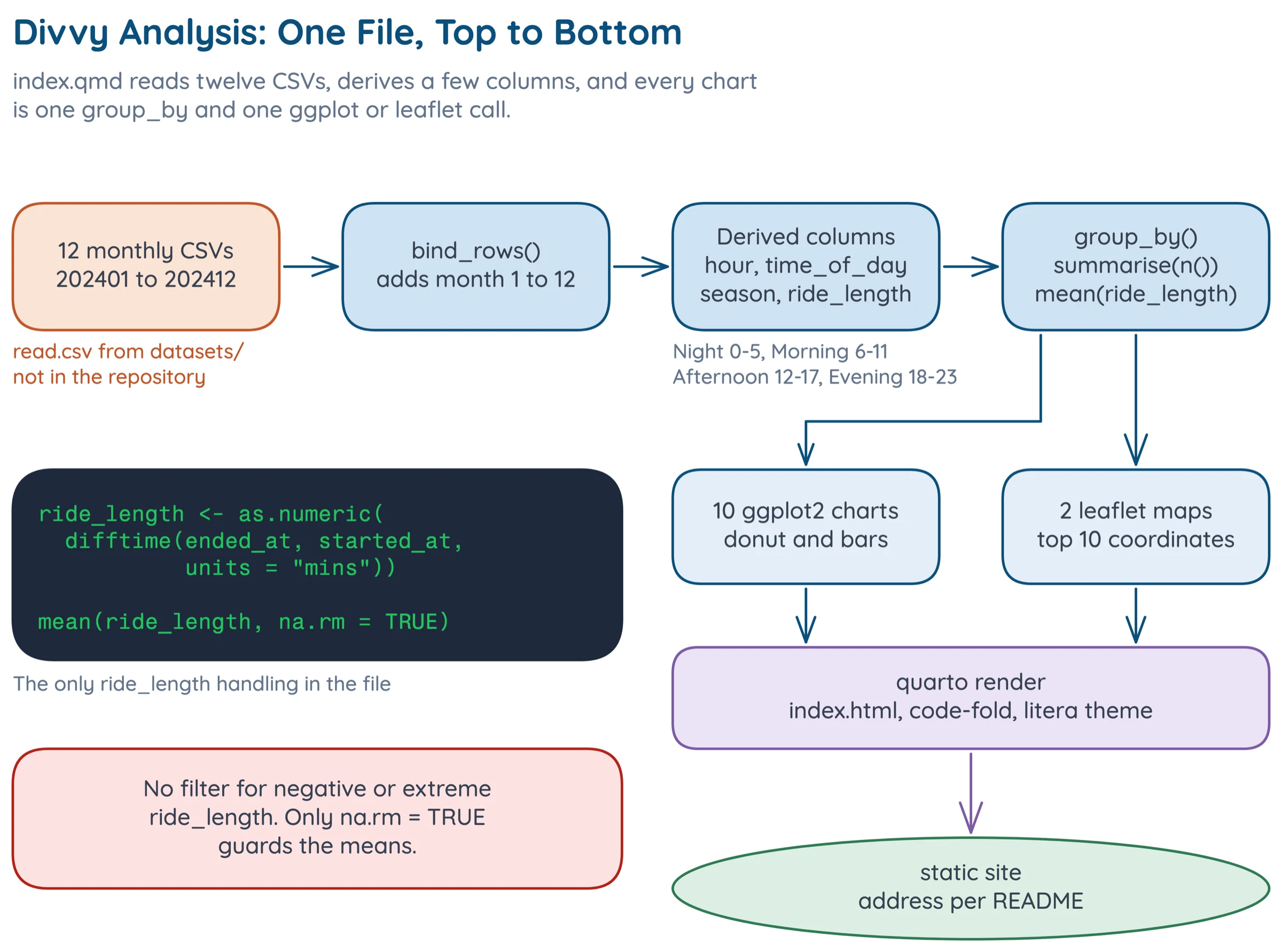
The rendered page carries ten charts and two maps.
Implementation
Reading and Combining
Each month is read with read.csv from a file named like 202401-divvy-tripdata.csv, and the twelve frames are stacked with bind_rows, tagging each with its month number.
df <- bind_rows( |
Derived Columns
The hour and the two time buckets are case_when calls on integer ranges.
df <- df |> |
The season column has the same shape on month. Ride length is as.numeric(difftime(ended_at, started_at, units = "mins")), the gap between end and start in minutes.
One Grouping per Chart
Every chart follows the same recipe. The average ride length by rider type is a group_by(member_casual), a mean(ride_length, na.rm = TRUE), and a bar chart with the rounded value printed above each bar. Counts by weekday, hour and month are n() over the matching key.
The rider-type donut is built by hand from ggforce::geom_arc_bar with start and end angles computed from cumulative proportions, and the number in its hole is round(nrow(df) / 1000000, 2) followed by "M Total Rides". That is where the 5.86M comes from.
Stations and Maps
The station bar charts lump station names to the top ten, drop missing names and the lumped "Other" group, and order the bars by count.
# abridged: the ggplot call that follows is omitted |
The Leaflet maps group by start_lat and start_lng, take slice_max(n = 10), and put the resulting points on a clustered marker layer.
Problems
The hard part of this project was deciding what a year of trip records can honestly support, and shaping every chart around that.
1. The Data Counts Trips, Not People
There is no user ID, so one person taking 300 rides counts 300 times. I built every chart around trips for that reason. Every number here is about trips, and "casual riders ride longer" really means "casual trips last longer". Nothing in the data says how many distinct people are behind either group.
2. A Mean Is Not a Typical Ride
The ride-length charts use the arithmetic mean of ended_at - started_at in minutes. Ride durations are right-skewed, so a few very long rides raise a mean without moving a median. I split the same mean three ways, by rider type, weekday and season, so no single bar carries the story. The 25.2 versus 12.8 gap is a gap in means, which is not the same as showing that a typical casual ride is twice as long as a typical member ride.
3. The Data Cannot Say Why
There is no trip purpose, distance or weather field, so I put that list of gaps at the top of the site. The charts show when and where people ride, never why. The obvious story for the ride-length gap, that casual riders are more often tourists and leisure riders on longer trips, is a guess this data cannot test. The same goes for the September peak: the data shows it, but has nothing that explains it.
Results
How Many Trips
The charts cover about 5.86 million trips in 2024. The seven weekday labels sum to 5,860,568, matching the 5.86M in the donut's hole.
Who Rides and on What
Electric and classic bikes carry almost all rides: electric bikes about 3.0 million, classic bikes about 2.7 million, and electric scooters about 0.15 million. Members are the majority on both classic and electric bikes, about 1.76M of 2.74M classic rides and 1.89M of 2.98M electric rides, or about 63% of electric rides. On the small scooter bar casual riders outnumber members, roughly 0.08M against 0.06M.
How Long
Casual riders average 25.2 minutes and members 12.8, a ratio of 1.97. Weekends are longer for everyone, at 20.9 minutes on Saturday and 21.4 on Sunday against 15 to 17 on weekdays.
By season, summer rides are longest and winter rides shortest: roughly 19.4 minutes for Summer, 17.4 for Spring, 15.6 for Fall and 14.3 for Winter.
When
Saturday is the busiest day, at 925,097 rides, and Sunday the quietest, at 787,201, just 987 rides below Monday. The gap between the busiest and quietest day is about 138,000 rides.
By hour, the day has a commuter shape. The chart peaks at 17:00 with roughly 600,000 rides, with 16:00 near 535,000 and 18:00 near 480,000, plus a smaller morning bump at 08:00 near 330,000. The minimum is overnight, at about 15,000 around hours 3 and 4.
By month, September is the peak, at about 820,000 rides, with July and August near 750,000. January is lowest at about 145,000 and December is about 178,000.
Where
One station dominates. Streeter Dr and Grand Ave leads both starts (about 66,000) and ends (about 67,000). The next tier is tight, running from DuSable Lake Shore Dr and Monroe St at about 44,000 down to Clinton St and Madison St at about 33,000.
The end-station chart has the same stations in a slightly different order.
What I Would Change
Report Medians Beside the Means
I would show medians next to every mean ride length. That would turn the 1.97 ratio from a gap in means into a claim about typical rides, or show that it does not hold up.
References
- John W. Tukey. Exploratory Data Analysis. Addison-Wesley, 1977.
- Hadley Wickham, Mara Averick, Jennifer Bryan, et al. Welcome to the Tidyverse. Journal of Open Source Software 4(43), 1686, 2019. doi:10.21105/joss.01686
- Hadley Wickham. ggplot2: Elegant Graphics for Data Analysis. Springer, 2016. link
- Joe Cheng, Barret Schloerke, Bhaskar Karambelkar, and Yihui Xie. leaflet: Create Interactive Web Maps with the JavaScript Leaflet Library. R package. link
- Posit PBC. Quarto: An Open-Source Scientific and Technical Publishing System. link
- Lyft Bikes and Scooters, LLC. Divvy Data License Agreement. link