O'Hare or Atlanta Tops Every Centrality Ranking

This project analyzes a sampled flight network and the interconnected airports within it. Using the descriptive techniques in Kolaczyk and Csárdi's Statistical Analysis of Network Data with R [1], I explore structural patterns in the graph and identify important airports and routes. It is one Quarto notebook in R with igraph [6]. A sample of 5,065 flights becomes a directed graph of 1,909 airports and 2,574 routes, and it has the hub-and-spoke shape airlines build: a small number of airports sit at the center with many connections, while most airports have only a few routes each.

The result I like most is how consistent the hubs are. I computed six centrality measures, each with its own idea of what "important" means, and every ranking is topped by either Chicago O'Hare or Atlanta. O'Hare leads on degree, closeness and betweenness. Atlanta leads on eigenvector centrality and on both hub and authority scores. The network is also disassortative, which means the big hubs connect to many small regional airports rather than to each other.

Why It Matters

When I fly to San Francisco, I always have to take a layover at Chicago O'Hare. That is not an accident. Most airlines want to reduce cost, and having only a few hubs makes repair and maintenance easier, so traffic gets routed through a handful of big airports.

Network analysis puts numbers on that intuition. Degree says which airports serve the most direct routes. Strength says where people are flying a lot more frequently. Betweenness says which airports sit on the shortest paths between everyone else, which is to say which ones are the layovers. Eigenvector centrality says which airports are connected to other important airports. Different centrality measures capture different aspects of importance, so seeing where they agree and where they don't says something about how the network is built.

This is a single notebook on a sample, not a model of world aviation. The sample includes a mix of major and regional airports, and the rankings describe the airports that ended up in it.

Technical Details

From Flights to a Graph

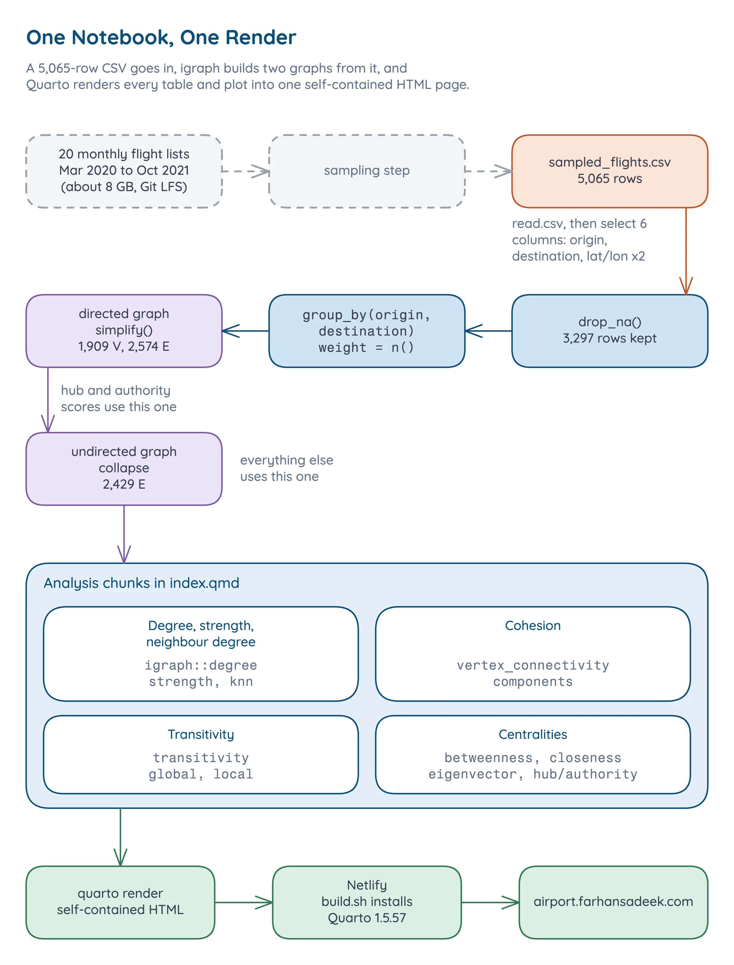
Each airport is a vertex, identified by its ICAO code (KORD is O'Hare, KATL is Atlanta, EDDF is Frankfurt). Each route from one airport to another is a directed edge, weighted by the number of sampled flights on it. I built both a directed graph and an undirected version that collapses the two directions of a route into one edge. The undirected graph, with 2,429 edges, carries most of the analysis. The directed one is used where direction matters, for hub and authority scores. Quarto renders the whole notebook to one self-contained page.

The sampled flights span 20 months, March 2020 to October 2021.

What Survives Into the Graph

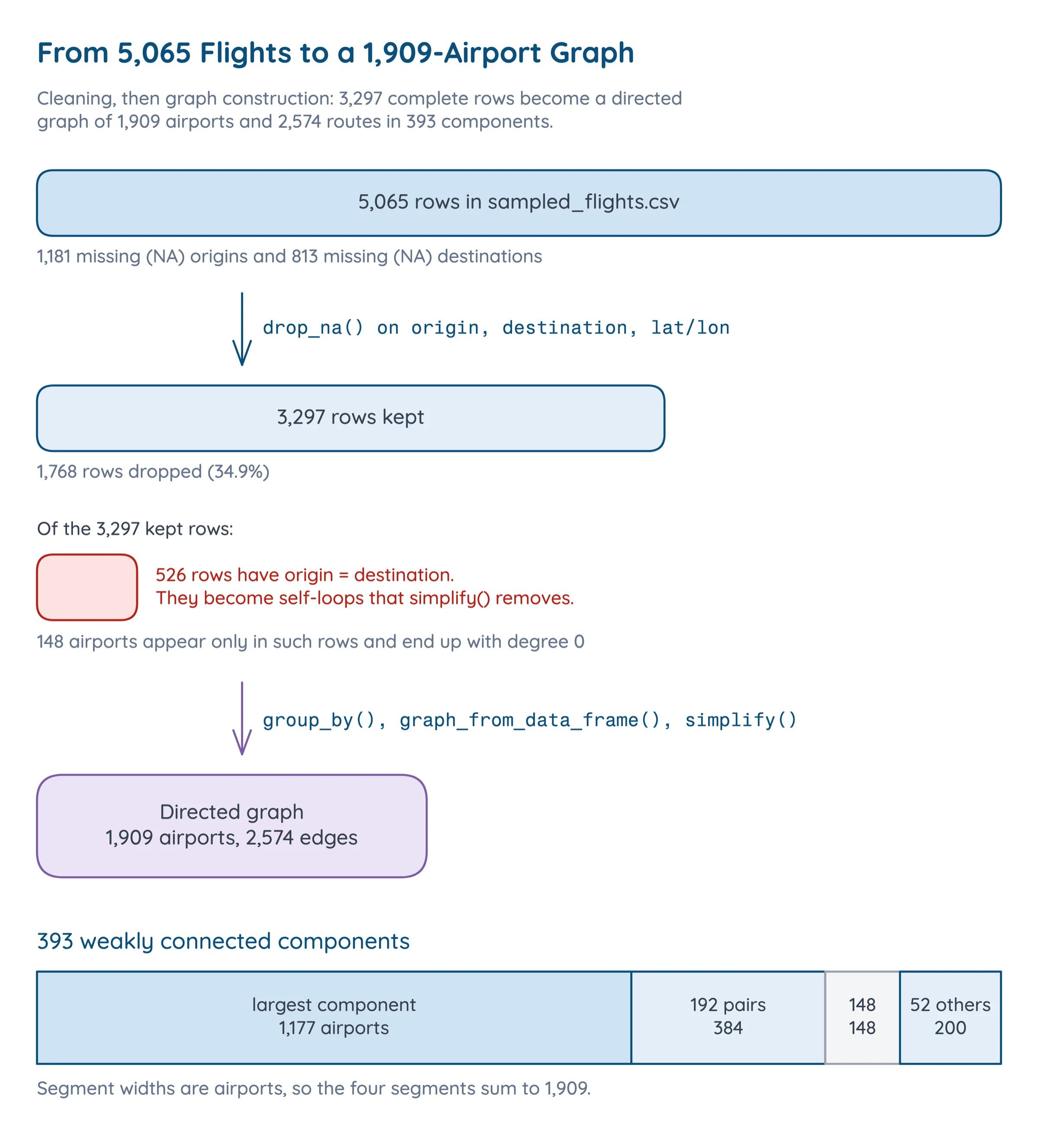
Not every row becomes an edge. A route needs both an origin and a destination, and a flight that departs and lands at the same airport is a self-loop, which a simple graph doesn't have.

Degree, Strength and Neighbours

The degree of an airport is the number of direct connections it has. In airline networks the degree distribution is usually highly skewed: a few major hubs have many connections, while most airports have only a few routes. Strength is the weighted version. It adds up the flights on each route, so it finds the airports people fly through most often, where degree finds the ones with the most destinations. Average neighbour degree is the mean degree of an airport's neighbours. Plotting it against the airport's own degree shows whether airports with lots of connections mostly link to other well-connected airports (assortative mixing), or to smaller, less connected ones (disassortative mixing).

Cohesion

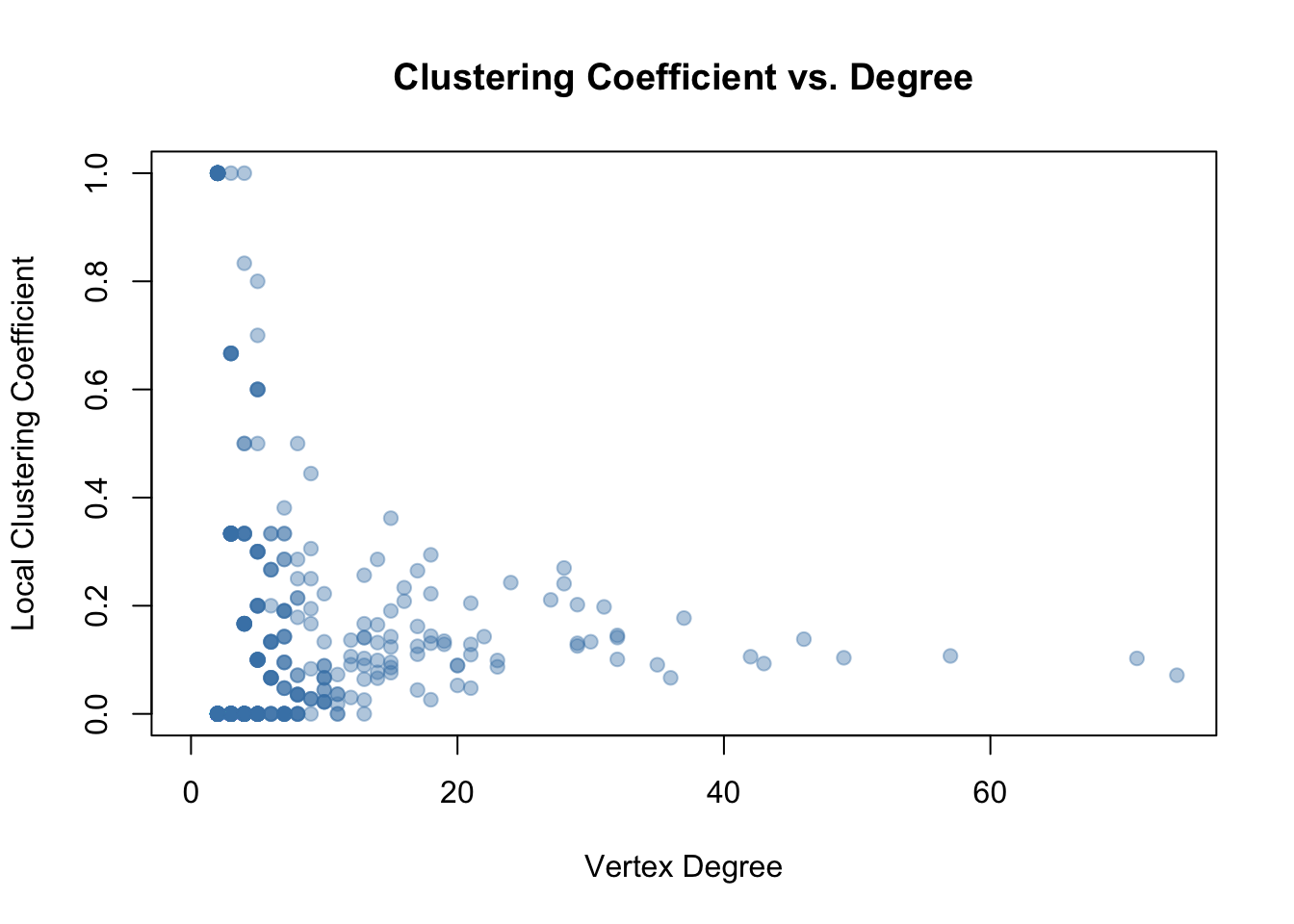
Vertex connectivity is the smallest number of airports whose removal disconnects the graph, and edge connectivity is the same count for routes. A graph that is already in pieces scores 0 on both. Transitivity, also called the clustering coefficient, measures the tendency for triangles to form. In an airport network, a triangle means that if airport A has direct flights to both B and C, then B and C also have a direct flight between them.

Centralities

Centrality measures identify the most important or influential nodes in a network, and each one captures a different notion of importance.

• Degree centrality is just the degree: which airports serve the most direct routes.
• Closeness is the inverse of the average shortest-path distance to every other airport. Airports with high closeness are well positioned to reach the entire network quickly. It is only defined within a connected piece of the graph, so I compute it on the largest component.
• Betweenness counts how many shortest paths between other pairs of airports pass through a given one [2], computed with Brandes' algorithm [3]. Airports with high betweenness are the critical choke points.
• Eigenvector centrality extends degree by weighting connections: being connected to well-connected airports matters more than being connected to poorly connected ones [4]. An airport is important if it is connected to other important airports.
• Hub and authority scores come from Kleinberg's HITS [5] on the directed graph. An airport is a good hub if it sends flights to many good authorities, and a good authority if it receives flights from many good hubs. In aviation terms, hubs are major departure points and authorities are major arrival destinations.

Implementation

Building the Network

The analysis starts from the 5,065 sampled flights. I selected only the columns needed for the analysis, constructed edge and vertex lists, and built both directed and undirected versions of the graph.

sampled_df <- sampled_df |>
  select(origin, destination, latitude_1, longitude_1, latitude_2, longitude_2) |>
  drop_na()

## Edge list: weighted by flight count per route
edges <- sampled_df |>
  group_by(origin, destination) |>
  summarise(weight = n(), .groups = "drop")

The vertex list comes from both ends of each flight, so every airport gets its coordinates. Then igraph builds the graph. The edge list is already aggregated by route, but simplification guarantees a simple graph and removes any self-loops.

flight_network <- graph_from_data_frame(d = edges, vertices = nodes, directed = TRUE)
flight_network <- simplify(flight_network, remove.multiple = TRUE, remove.loops = TRUE)

## Undirected version for symmetric analyses
flight_undirected <- igraph::as.undirected(flight_network, mode = "collapse")

summary(flight_network) reports DNW- 1909 2574: directed, named, weighted, 1,909 vertices and 2,574 edges.

Vertex Characteristics

Each characteristic is a few lines of igraph plus a plot. Average neighbour degree, for example, comes from knn(), plotted on log axes against degree.

a.nn.deg.flight <- knn(flight_undirected, V(flight_undirected))$knn
plot(igraph::degree(flight_undirected), a.nn.deg.flight,
     log = "xy",
     col = adjustcolor("steelblue", alpha.f = 0.5),
     pch = 19)

Centralities

Each centrality is a one-line igraph call, a sort, and a kable of the top ten. Closeness first pulls out the largest component with induced_subgraph().

lcc <- induced_subgraph(flight_undirected,
                        which(comp$membership == which.max(comp$csize)))
close_cent <- igraph::closeness(lcc)

betw_cent <- igraph::betweenness(flight_undirected, normalized = TRUE)
top_betweenness <- sort(betw_cent, decreasing = TRUE)[1:10]

Hub and authority scores use hub_score() and authority_score() on the directed graph. To compare the measures, I put degree, betweenness, eigenvector centrality and strength for every airport into one data frame and drew a pairs() scatter matrix.

Problems

1. A 1,909-Airport Graph Is Unreadable as a Raw Plot

In a network this large, raw plots become unreadable. I wanted a picture that shows the hub-and-spoke structure at a glance, so the visualization drops the edges and packs one circle per airport with packcircles. Size is betweenness, colour is degree from very low to very high, and only the top 10% by betweenness get a label. Airports with zero betweenness can't be sized, so the plot keeps only the airports with nonzero betweenness.

packing <- circleProgressiveLayout(df$centrality, sizetype = "area")
df <- cbind(df, packing)
dat.gg <- circleLayoutVertices(packing, npoints = 100)

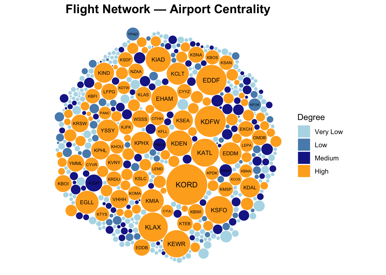
From this visualization I can see the hub-and-spoke structure that airlines follow. A small number of airports, in red and orange, sit at the center with many connections, while the majority of airports cluster around the periphery with only a few routes each.

2. Degree Bins Collide When Degree Varies Little

The colours come from cutting degree into five quantile bins. That breaks when degree has little variation: two quantiles can land on the same value, and cut() refuses duplicate break points. The fix is to keep only the unique breaks and cap the bin index at five, so the palette always has a colour for every bin.

deg_breaks <- unique(quantile(df$degree, probs = seq(0, 1, length.out = 6), na.rm = TRUE))
if (length(deg_breaks) >= 2) {
  df$deg_bin <- as.integer(cut(df$degree, breaks = deg_breaks, include.lowest = TRUE, labels = FALSE))
  df$deg_bin <- pmin(df$deg_bin, 5)  # cap at 5 for color_pal
} else {
  df$deg_bin <- 1L
}

3. Closeness Needs a Connected Graph

Closeness is an average distance to every other airport, and the distance to an airport in a different component is infinite. With 393 components, closeness on the full graph doesn't mean much. Restricting it to the largest component, 1,177 airports, gives a closeness that means something, at the cost of saying nothing about the airports outside it.

Results

The Network Is Sparse and in Pieces

Property	Value
Airports (vertices)	1,909
Flight routes (edges), directed / undirected	2,574 / 2,429
Simple graph	yes
Weakly / strongly connected	no / no
Weakly connected components	393
Size of largest component	1,177
Isolates (degree 0)	148
Diameter (unweighted)	19
Average path length	5.4329
Edge density	0.000707
Vertex / edge connectivity	0 / 0
Global / average local transitivity	0.1209 / 0.105

Vertex and edge connectivity are both 0 because the graph is already in 393 pieces, so nothing has to be removed to disconnect it. The largest component holds 1,177 airports. In a hub-and-spoke network these values are often low anyway, because removing just a few critical hubs would collapse the network.

Transitivity is low too, at 0.1209 globally and 0.105 on average per airport.

Most Airports Have One Route, a Few Have Dozens

The degree distribution is very skewed. Most airports don't have very many connections, but the hubs have a lot. Of 1,909 airports, 1,114 have degree 1 and 1,523 have degree 2 or less, while O'Hare has 74.

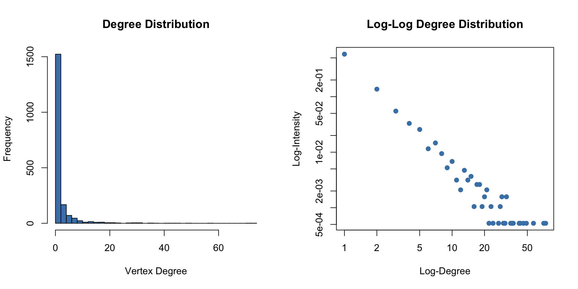
The log-log plot shows a linear relationship in the tail, which is an indication of a power-law or scale-free degree distribution [7]. That fits the cost argument, since airlines concentrate routes on a few hubs.

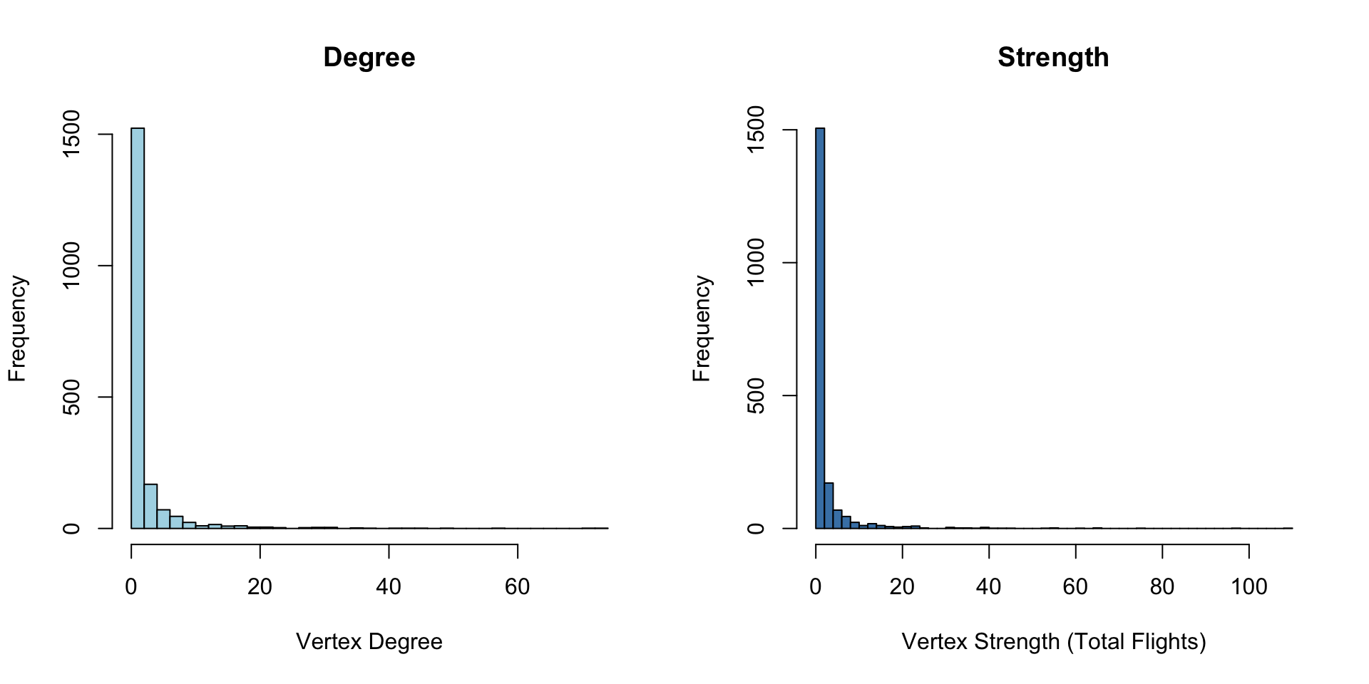
Strength, which counts flights instead of routes, tells the same story more strongly. Both distributions are right-skewed, but the strength distribution has an even longer tail. The major hubs have more destinations, and their flights are more frequent too.

Hubs Connect to Small Airports

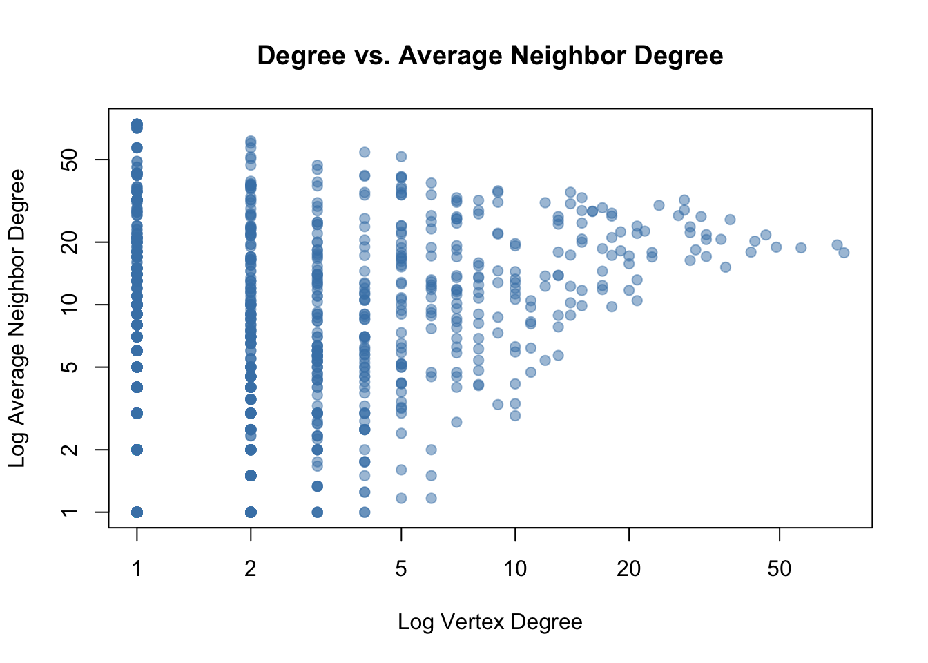
The plot shows a negative trend: higher-degree airports tend to be connected to neighbours with lower average degree. This is textbook disassortative mixing, which is characteristic of hub-and-spoke transportation networks. The big hubs connect to many small regional airports, which in turn have the hub as their most prominent neighbour. This contrasts with social networks, which are typically assortative: popular people befriend other popular people.

The Same Airports Win Every Ranking

Measure	Top five
Degree	KORD 74, KATL 71, KDFW 57, KDEN 49, KLAX 46
Closeness (largest component)	KORD 0.000260, KDFW 0.000250, KEWR 0.000246, KSFO 0.000245, KATL 0.000244
Normalized betweenness	KORD 0.0663, KDFW 0.0384, EDDF 0.0367, KLAX 0.0342, KATL 0.0313
Eigenvector	KATL 1.000, KORD 0.777, KSEA 0.722, KLAS 0.674, KLAX 0.663
Hub score	KATL 1.000, KORD 0.861, KSEA 0.847, KLAX 0.805, KDEN 0.760
Authority score	KATL 1.000, KORD 0.707, KLAS 0.588, KDFW 0.561, KSEA 0.556

Chicago O'Hare or Atlanta is first on every one of the six measures, and Dallas-Fort Worth, Denver and Los Angeles keep showing up behind them. By degree, Dallas-Fort Worth and Charlotte are among the major hubs in the network, with Charlotte sixth at 43 routes.

For closeness, as expected, Dallas is high up the list, in second. Newark, San Francisco, Miami and Amsterdam move into the top ten, and Charlotte drops out of it. I think the most likely reason is that many of Charlotte's flights end in the network rather than following on to more destinations.

Betweenness has the major hubs on top again, meaning they are the airports that connect flights from one airport to another. That is my San Francisco trip: I always lay over at O'Hare, and O'Hare's betweenness of 0.0663 is about 1.7 times the next airport's. Frankfurt and Amsterdam are third and eighth, and Washington Dulles is tenth at 0.0254.

Eigenvector centrality brings Seattle and Las Vegas up to third and fourth, because they are connected to other well-connected airports. Hub scores follow the busiest departure points, and Charlotte reappears ninth there.

I was surprised that Detroit only just makes the hub list, tenth at 0.557, because Detroit is a major Delta hub. One reason I can think of is that Detroit is not as sought-after a destination as Chicago, Dallas, San Francisco or New York. But it seems like Detroit is a good location for a connecting hub.

How the Measures Agree

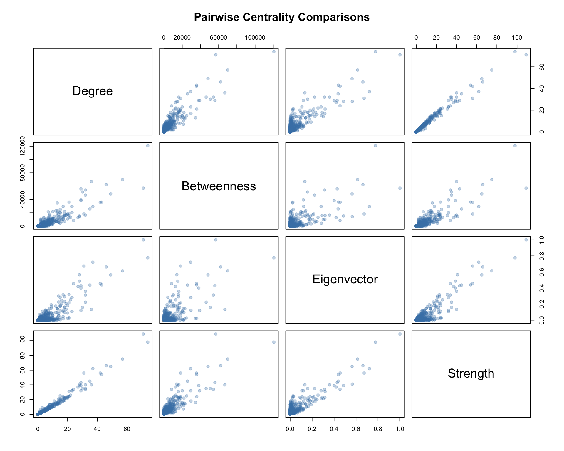
All the centrality measures are positively correlated, so the major hubs tend to score high across all of them. Strength and degree are almost the same measure here, with a Spearman correlation of 0.984, and betweenness tracks both closely, at 0.917 against degree and 0.898 against strength. Eigenvector centrality is the one that goes its own way, at 0.565 to 0.672 against the others, because it rewards being attached to important airports rather than having many routes. Betweenness can be high for airports that serve as critical bridges even if they don't have many direct connections.

References

1. Eric D. Kolaczyk, Gábor Csárdi. Statistical Analysis of Network Data with R, 2nd edition. Springer, 2020. doi:10.1007/978-3-030-44129-6
2. Linton C. Freeman. A Set of Measures of Centrality Based on Betweenness. Sociometry 40(1), 35–41, 1977. doi:10.2307/3033543
3. Ulrik Brandes. A Faster Algorithm for Betweenness Centrality. Journal of Mathematical Sociology 25(2), 163–177, 2001. doi:10.1080/0022250X.2001.9990249
4. Phillip Bonacich. Factoring and Weighting Approaches to Status Scores and Clique Identification. Journal of Mathematical Sociology 2(1), 113–120, 1972. doi:10.1080/0022250X.1972.9989806
5. Jon M. Kleinberg. Authoritative Sources in a Hyperlinked Environment. Journal of the ACM 46(5), 604–632, 1999. doi:10.1145/324133.324140
6. Gábor Csárdi, Tamás Nepusz. The igraph Software Package for Complex Network Research. InterJournal Complex Systems, 1695, 2006. link
7. Aaron Clauset, Cosma Rohilla Shalizi, M. E. J. Newman. Power-Law Distributions in Empirical Data. SIAM Review 51(4), 661–703, 2009. doi:10.1137/070710111